Regression With Scikit Learn (Part 1)

This post will look into how we can create a linear regressor to make predictions about continuous target variables.

Source code can be found on my GitHub repo okeeffed/regression-with-scikit-learn.

Prerequisites

Getting started

Let's create the regression-with-scikit-learn directory and install the required packages.

# Clone and add a Python notebook
$ git clone okeeffed/supervised-learning-with-scikit-learn-template regression-with-scikit-learn
$ cd regression-with-scikit-learn
$ touch docs/regression.ipynb
copy

At this stage, we are ready to add in a linear regressor.

Exploring the Boston dataset

In this example, we will use the Boston housing dataset to predict the price of a house.

In our file docs/regression.ipynb, we can add the following:

from sklearn.datasets import load_boston

boston = load_boston()
print(boston.DESCR)
copy

The above will print out the dataset description.

Under :Number of Attributes:, we see the description "13 numeric/categorical predictive. Median Value (attribute 14) is usually the target."

It is the MEDV that we will be trying to predict.

In our second cell, add the following:

X = boston.data
y = boston.target

# Create the dataframe
import pandas as pd

df = pd.DataFrame(X, columns=boston.feature_names)
print(df.head()) # print the first 5 rows
copy

Here we are assigning the X and y variables to the boston dataset based on features and target respectively.

From there, we are creating a data frame with the features and target with panda.

Printing the head shows us the first five rows:

CRIM    ZN  INDUS  CHAS    NOX     RM   AGE     DIS  RAD    TAX  \
0  0.00632  18.0   2.31   0.0  0.538  6.575  65.2  4.0900  1.0  296.0
1  0.02731   0.0   7.07   0.0  0.469  6.421  78.9  4.9671  2.0  242.0
2  0.02729   0.0   7.07   0.0  0.469  7.185  61.1  4.9671  2.0  242.0
3  0.03237   0.0   2.18   0.0  0.458  6.998  45.8  6.0622  3.0  222.0
4  0.06905   0.0   2.18   0.0  0.458  7.147  54.2  6.0622  3.0  222.0

   PTRATIO       B  LSTAT
0     15.3  396.90   4.98
1     17.8  396.90   9.14
2     17.8  392.83   4.03
3     18.7  394.63   2.94
4     18.7  396.90   5.33
copy

This information can give us some insight to what the data will look like.

We want to create a linear regressor to predict the MEDV variable based on the number of rooms, so we will need to adjust our X to only pass the one dimension.

X_rooms = X[:, 5]

# We need to reshape our data from a 1d to a 2d array
# For more info, see https://jakevdp.github.io/PythonDataScienceHandbook/02.02-the-basics-of-numpy-arrays.html#Reshaping-of-Arrays
# Also see https://numpy.org/doc/stable/reference/generated/numpy.reshape.html
X_rooms = X_rooms.reshape(-1, 1)

df = pd.DataFrame(X_rooms, columns=[boston.feature_names[5]])
print(df.head()) # print the first 5 rows
copy

The above code will only take the data for the rooms feature and reshape it to a 2d array.

The resulting data frame is the following:

RM
0  6.575
1  6.421
2  7.185
3  6.998
4  7.147
copy

Visualizing the data

We can take the variables we have assign X_rooms and y to visualize the data.

In a new cell, add the following:

import matplotlib.pyplot as plt

plt.scatter(X_rooms, y)
plt.ylabel('Value of house /1000 ($)')
plt.xlabel('Number of rooms')
plt.show()
copy

Executing that code gives us the following:

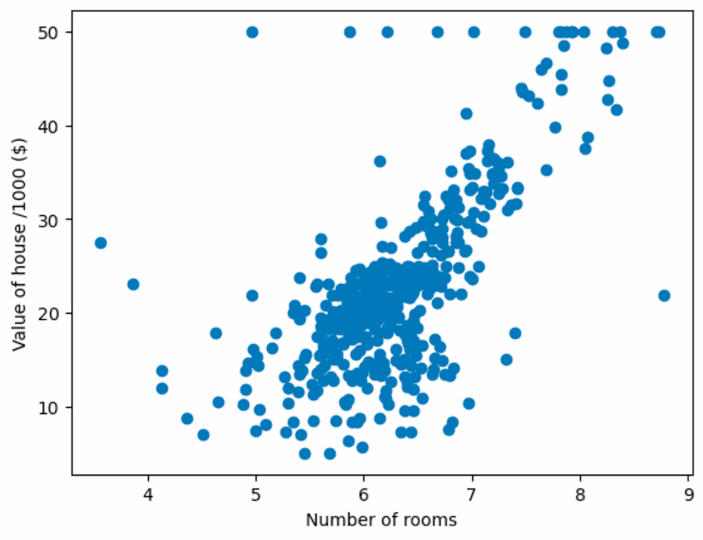
Value of house /1000 ($) vs Number of rooms

As you could imagine intuitively, the price of the house rises as the number of rooms increase.

Creating a regressor to predict a continuous target variable

Finally, we can build a linear regressor to predict the MEDV variable.

import numpy as np
from sklearn.linear_model import LinearRegression

reg = LinearRegression()

# Fit the regressor to the data
reg.fit(X_rooms, y)

prediction_space = np.linspace(min(X_rooms), max(X_rooms)).reshape(-1, 1)

# Re-create the scatter plot
plt.scatter(X_rooms, y)
plt.ylabel('Value of house /1000 ($)')
plt.xlabel('Number of rooms')

# We add the prediction to the plot as a black line
plt.plot(prediction_space, reg.predict(prediction_space), color='black', linewidth=3)
plt.show()
copy

This provides us with a visual line of the predicted values on the linear regressor.

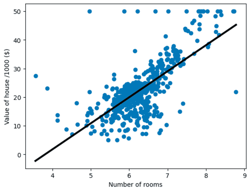
Adding the line to the data

Summary

Today's post was an introduction to regression with Scikit Learn. We used the Boston dataset to predict the MEDV variable.

Moving forward, we will dive deeper into linear regression theory apply this to a test/train split. Then we will look into cross-validation, as well a regularization.

Resources and further reading

Photo credit: pawel_czerwinski